The Transformer Network for the Traveling Salesman Problem 2022-10-30 组合优化 暂无评论 78 次阅读 ## 下载 论文: [[2103.03012v1] The Transformer Network for the Traveling Salesman Problem (arxiv.org)](https://arxiv.org/abs/2103.03012v1) 代码: [xbresson/TSP_Transformer: Code for TSP Transformer (github.com)](https://github.com/xbresson/TSP_Transformer) ## 前置知识 ### Self-attention #### 用处 和RNN一样能处理序列信息 并行 <img src="https://pic.lass.work/i/2022/10/30/10hgw75-0.png" style="zoom:80%;" /> #### 实现 - embeding之后,计算q,k,v  - q与所有ki做attention 为了防止内积过大,因此除以d的平方根。  - softmax  - 与所有vi相乘,求和得到输出  - 以上均可转换为矩阵运算  #### 如何处理变长数据 - RNN如何处理变长数据  每个时间步的RNN块,权重共享,输入序列多长,就加多少RNN块 - Self-attention如何处理变长数据 self-attention的参数只在Wq、Wk、Wv,它们和输入序列长度无关, ### Multi-head Self-attention Multi-Head Attention 是由多个 Self-Attention 组合形成的,最后拼接在一起  ### Transformer  #### 位置编码Positional Encoding 因为 Transformer 不采用 RNN 的结构,而是使用全局信息,不能利用单词的顺序信息,而这部分信息对于 NLP 来说非常重要。所以 Transformer 中使用位置 Embedding 保存单词在序列中的相对或绝对位置。  位置 Embedding 用 **PE**表示,**PE** 的维度与单词 Embedding 是一样的。PE 可以通过训练得到,也可以使用某种公式计算得到。  其中,pos 表示单词在句子中的位置,d 表示 PE的维度 (与词 Embedding 一样),2i 表示偶数的维度,2i+1 表示奇数维度 (即 2i≤d, 2i+1≤d)。使用这种公式计算 PE 有以下的好处: - 使 PE 能够适应比训练集里面所有句子更长的句子,假设训练集里面最长的句子是有 20 个单词,突然来了一个长度为 21 的句子,则使用公式计算的方法可以计算出第 21 位的 Embedding。 - 可以让模型容易地计算出相对位置,对于固定长度的间距 k,**PE(pos+k)** 可以用 **PE(pos)** 计算得到。因为 Sin(A+B) = Sin(A)Cos(B) + Cos(A)Sin(B), Cos(A+B) = Cos(A)Cos(B) - Sin(A)Sin(B)。 将单词的词 Embedding 和位置 Embedding 相加,就可以得到单词的表示向量 **x**,**x** 就是 Transformer 的输入。  #### encoder ##### 2.1 Add & Norm **Add**指 **X**+MultiHeadAttention(**X**),是一种残差连接,通常用于解决多层网络训练的问题,可以让网络只关注当前差异的部分,在 ResNet 中经常用到: 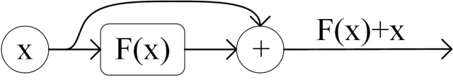 **Norm**指 Layer Normalization,通常用于 RNN 结构,Layer Normalization 会将每一层神经元的输入都转成均值方差都一样的,这样可以加快收敛。 Batch Normalization 的处理对象是对一批样本, Layer Normalization 的处理对象是单个样本。Batch Normalization 是对这批样本的同一维度特征做归一化, Layer Normalization 是对这单个样本的所有维度特征做归一化。  >[batchNormalization与layerNormalization的区别 - 知乎 (zhihu.com)](https://zhuanlan.zhihu.com/p/113233908) ##### 2.2 Feed Forward Feed Forward 层比较简单,是一个两层的全连接层,第一层的激活函数为 Relu,第二层不使用激活函数,对应的公式如下。 <img src="https://pic2.zhimg.com/80/v2-47b39ca4cc3cd0be157d6803c8c8e0a1_720w.webp" style="zoom:50%;" /> **X**是输入,Feed Forward 最终得到的输出矩阵的维度与**X**一致。  #### decoder 与 Encoder block 相似,但是存在一些区别: - 包含两个 Multi-Head Attention 层。 - 第一个 Multi-Head Attention 层采用了 Masked 操作。 - 第二个 Multi-Head Attention 层的**K, V**矩阵使用 Encoder 的输出矩阵C进行计算,而**Q**使用上一个 Decoder block 的输出计算。 - 最后有一个 Softmax 层计算下一个翻译单词的概率。 ##### 3.1 mask 在得到 QK<sup>T</sup>之后需要进行 Softmax,计算 attention score,我们在 Softmax 之前需要使用**Mask**矩阵遮挡住每一个输入向量之后的信息,得到 Mask QK<sup>T</sup>后再进行softmax,每个向量与它后面的向量的attention score都是0。  ##### 3.2 自回归与非自回归   How to decide the output length for NAT decoder? - Another predictor for output length - Output a very long sequence, ignore tokens after END ## 论文的网络        ## 代码 ### 数据 强化学习,不是监督训练 数据集是随机生成的 ### 网络 ### 训练/loss >Wouter Kool, Herke V an Hoof, and Max Welling. 2018. Attention, learn to solve routing problems! arXiv preprint arXiv:1803.08475 (2018). Loss:the expectation of the cost L(π) (tour length for TSP)  We optimize Loss by gradient descent, using the REINFORCE (Williams, 1992) gradient estimator with baseline b(s):  We propose to use a rollout baseline in a way that is similar to self-critical training by Rennie et al. (2017), but with periodic updates of the baseline policy. It is defined as follows: b(s) is the cost of a solution from a deterministic greedy rollout of the policy defined by the best model so far. A stronger algorithm defines a stronger baseline, so we compare (with greedy decoding) the current training policy with the baseline policy at the end of every epoch, and replace the parameters θBL of the baseline policy only if the improvement is significant according to a paired t-test (α = 5%), on 10000 separate (evaluation) instances.   标签: 组合优化 本作品采用 知识共享署名-相同方式共享 4.0 国际许可协议 进行许可。
评论已关闭